Abstract

Exoplanet research is currently going through a renaissance. The planets existing outside of our Solar system are the exoplanets. In scientific news, you often hear that ”water” has been found in so and so ”X” planet. There are signs of methane in an Earth-like planet showing signs of life. How do scientists detect the elements in the atmosphere of an exoplanet? How do they retrieve the different parameters of the atmosphere? This article will briefly overview the retrieval processes, understanding of spectroscopy, and how the temperature and chemical composition of the atmosphere change the transmission spectrum.

Introduction

Atmospheric retrieval is the inference of the atmospheric properties of an exoplanet given an observed spectrum. We can go beyond detecting gases in exoplanet atmospheres to measure how much of each chemical resides in the atmosphere. Extracting this detailed information from an observed spectrum is called atmospheric retrieval. The atmospheric properties include the chemical composition, temperature structure atmospheric circulation, and clouds/hazes, all of which leave their imprints on the spectrum. The retrieved properties can, in turn, provide insights into the various atmospheric physical and chemical processes as well as into their formation history. So, without any further delay let us dive into the world of exoplanets and explore what spectroscopy is and why it is necessary in retrieving the planets’ properties.

Spectroscopy

Spectroscopy is one of the most powerful tools of an astronomer: the splitting of light into its individual colors (wavelengths). The sky is blue as the molecules present in our atmosphere interacts strongly with the sun’s radiation in the higher energy(lower wavelength) than in the lower energy and thus causing it to scatter in different directions. Similarly, different colors of light are treated differently by the gases making up exoplanet atmospheres, with some colors absorbed while others can pass through. This can be better understood through the Radiative Transfer equation which is a whole new topic which I will not be covering in this article. But, for brief introduction, the radiative transfer equation explains the interaction of light in different wavelength(colors) with different molecules and returns the intensity values at different layers of the atmosphere. Let us understand transmission spectroscopy.

Transmission Spectroscopy

In the modern age with the help of strong telescopes such as HST and JWST, we are able to get the intensity of the radiation of a star. Now, if a planet orbiting that star comes in the path of the line of sight, it obstructs some of the intensity given by the star and acts as an opaque object, thus, decreasing the overall intensity. The larger the planet, the larger is the drop in the intensity. If our planet has an atmosphere, which composes of different molecules that interact with each wavelength of the stars light differently(absorbs, emits, or scatters) this may not cause complete blockage of light. From the apriori knowledge of how different compounds interact with light in different wavelength on our planet, we know that different compounds have a characteristic wavelength at which they strongly absorb. Let me break this down in a simpler manner.

Case 1: No atmosphere

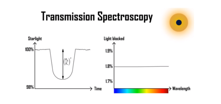
The top right of the image shows the transit of an exoplanet in front of its host star. The left part of the image shows the dip in the intensity of the light. The right part of the image shows the plot between the light blocked (transit depth) and the wavelength of light.

In the left part of the image the intensity of the starlight starts to decrease when the exoplanet just enters the line of sight and reaches the minimum when it is completely blocking(opaque) the starlight continues to stay in the minimum until it exits the line of sight. This length from the maximum intensity to the minimum intensity is known as the transit depth and is equal to (Rp/Rs) 2 where Rp is the radius of the planet and Rs is the radius of the host star.

Let us say that our transiting exoplanet has no atmosphere(like Mercury) which means it has no molecules, no gases(like a ball of rock) etc. which means that there is no additional layer of gases that is blocking the light and hence we see a flat line which means there is constant fraction of light is blocked(all the colors of light are blocked equally).

Case 2: H2/He in atmosphere

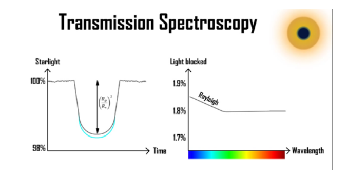
Adding H2/He in the atmosphere

When we add an atmosphere to the planet, in this case, say H2/He a phenomenon known as Rayleigh scattering occurs where short wavelengths, or high energy blue light bounces about or scatters around the atmosphere, so the amount of light blocked appears to slope upwards in the blue light which we call the Rayleigh slope. This means that the planet appears to be bigger in smaller wavelength regions and when we look at the light at higher wavelengths, we do not have the extra layer of the atmosphere and hence the light blocked in this higher wavelength region is the same as the original.

Case 3: Presence of Alkali metals

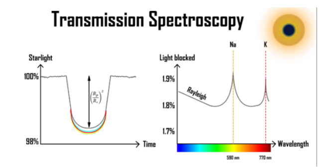
Characteristic wavelength of alkali metals like Sodium and Potassium

Sodium has a strong absorption feature at 590 nanometers in yellow light, which means that if you observe the planet in yellow light, the atmosphere is actually opaque and the planet appears slightly larger and the transit depth in yellow light increases and hence the amount of light blocked peaks in this region. Similarly if the atmosphere has potassium in the atmosphere, then we see the planet becoming larger again in red light around 770 nanometers.

This is the story in the visible wavelength. If we want to know what molecules are present in the atmosphere, we will need to expand the wavelength spectrum in the infrared region.

Transmission Spectrum

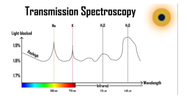
Expanding the spectrum

In the infrared region, water has a strong absorption feature. Now, if we look at the other wayround, at these wavelengths, if the planet appears to be bigger we can estimate that this might be caused by the presence of water molecules in the atmosphere of the planet.

Free Parameters

There are several factors that affect the Transmission spectrum. Hence we develop several models and try to match the observed data set to retrieve the data of the atmosphere. These factors comprise of parameters such as profiles of pressure (P), temperature (T), density (ρ), concentrations (fi) of individual chemical species, cloud/haze profile, if any, etc., and computing the radiative transfer for the given atmospheric structure. Briefly, the radiative transfer equation helps us to solve for the intensities in each layer of the atmosphere which in turn computes the Pressure and Temperature considering the absorption, emission and scattering feature of the molecules present in the atmosphere.

Here, I is the intensity, lambda is the wavelength of the light, τ is the optical depth(defined as the product of concentration and opacity of the molecule: amount it scatters or transmits), mu is the cosine of the zenith angle and S is the source function.

Bayesian Inference

Stating the Bayes Theorem:

Here, \(θ_i\) denotes the set of parameters of an atmospheric model, and \(d\) denotes the data, such as an observed spectrum. \(p(θ_i—d)\) is the posterior probability distribution of the model parameters given the data, and \(p(d—θ_i)\) is the probability of data given a parameter set. \(p(θ_i)\) is the prior probability distribution of the model parameters independent of the data. \(p(d)\) aka the evidence is the likelihood of the data set. The goal in Bayesian inference is to determine the posterior distributions \(p(θ—d)\) of the model parameters for a given dataset and considering any prior knowledge of the parameters.

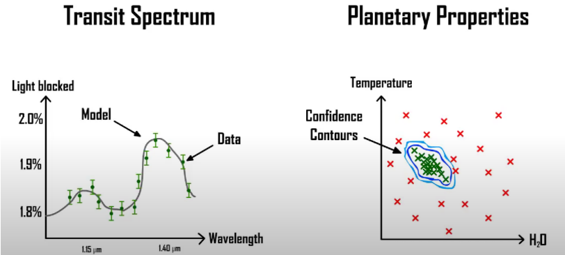
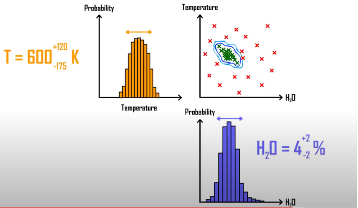
MCMC(Monte Carlo Markov Chain) for a set of two parameters H2O and Temperature

For instance, let us consider two free parameters, the concentration of water, and the Temperature of the atmosphere. As you can see in the figure, the left part shows the data with green points, whereas the model based on all the physics applied with these two parameters(in this case for simplicity) is the curve. Now, say for a particular value of Temperature and water my model fits the data, I mark this coordinate with a green cross as shown in the right side of the figure. If I drastically increase the Temperature this model will not fit the data and is off and I will mark it with a red cross mark. Now I have different combinations of H2O concentrations and Temperature for which my model is close enough to the data set or far off. I name the region of all the green crossed points as ”Confidence Contours”. This is the region where the values of these two parameters has the highest probability of matching my model with the data set.

Retrieving the Parameters

Here you are mapping the the best models on the probability distribution to estimate the best model of the atmosphere of the exoplanet. But this is a simple example with just two parameters. In reality, there are 10+ parameters accounting to 10^10 models which requires the best of the optimal computation techniques and super fast GPUs. I would like to end this discussion with showing the real atmospheric retrieval model showing the best fit model which might look messy but the basic idea remains the same.

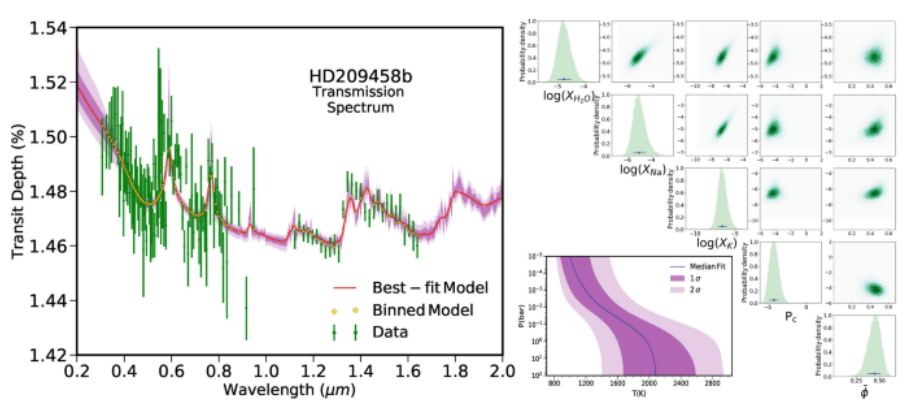
A real Retrieval model of an exoplanet HD209458b with 10 parameters

Conclusion

In this article, we briefly discussed the Bayesian analysis to find the best-fit model considering various parameters that can be found by the radiative transfer equation given the data set. The interaction of light with different molecules in different wavelengths and how their absorption features in their characteristic wavelengths help us to determine the presence or absence of their concentration in the atmosphere has also been discussed. It is fascinating how we can understand the composition and characteristics of an atmosphere light years away from us just by minimal information, that is, the intensity of the host star detected by telescopes by sitting in front of our computers. This will give us profound information on the physiochemical processes, the history of planetary formation mechanisms, and the signs of habitability and life beyond the Earth.

References

1) Ryan Macdonald. Transmission spectrum. https://distantworlds.space/overview, 2021. Accessed: 2024-07-11.

2) Ryan Macdonald. Atmospheric retrieval of exoplanets. https://youtu.be/ZnLg4YFMfDQ? feature=shared, 2021. Accessed: 2024-07-11.

3) Nikku Madhusudhan. Atmospheric retrieval of exoplanets. arXiv preprint arXiv:1808.04824, 2018.